1D Hydraulic Modelling
Hydrodynamic Modelling using HEC-RAS

Part 1: set-up and analysis of a simple channel model

This page describes the 1st part of the 3rd assignment.

The 1st part of the assignment deals with a simple channel model as preparation for more complex modelling tasks in part2. This page describes the main steps to update a basic steady HEC-RAS model similiar as used in assignment 2 towards a first unsteady model. The main steps to set-up such HEC-RAS model are described in the related tutorial of assignment 2.

Basic steady model properties:

homogeneous channel of 5000m length
prismatic rectangular cross section of 50m width and 10m height
known water surface elevation upstream and downstream: 4 m
estimated channel roughness of 30 (Strickler) / 0.0333 (Manning).
no slope
no weir

Step 1: Basic steady HEC-RAS model

Please download the basic steady model from the course server: Extract the model to a new folder. Run the steady simulation and analyse the results by physical interpretation.

Step 2: Set-up 1st unsteady model

Please create a unsteady simulation for the basic model.

same geometry as the steady model
same channel roughness as the steady model
simulation window: 2 hours with 1 minute time step
initial conditions: no flow, constant water level of 4 m
boundary conditions: upstream known water level h(t) = 4 m
boundary conditions: downtream known discharge q(t) = 0 m3/s (no flow, vertical wall)

step	action/screenshot thumbnails with links to full size images	remark
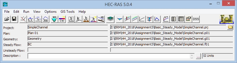
1.	start HEC-RAS project form:	open the basic steady model file SimpleChannel.prj
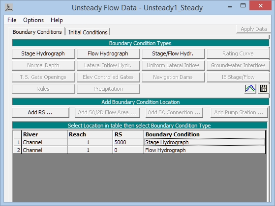
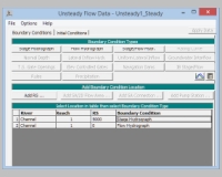
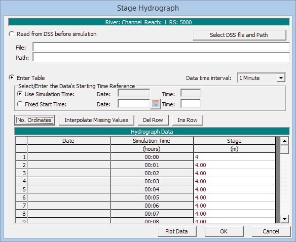
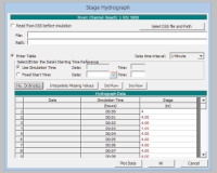
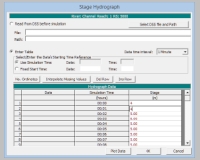
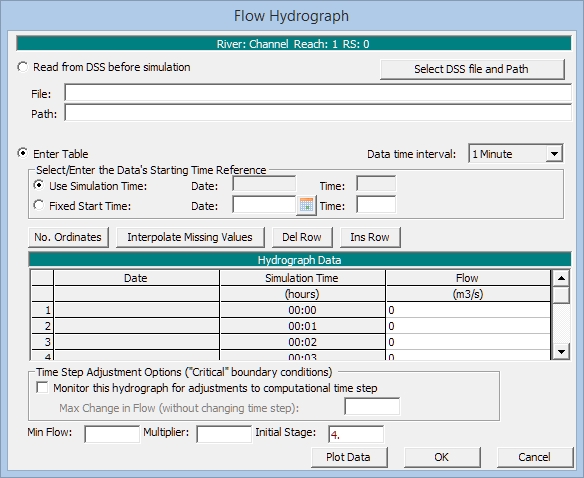
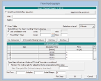
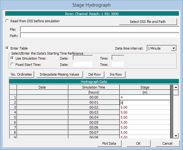
2.	open and edit Unsteady Flow Data unsteady flow data form: stage hydrograph form: flow hydrograph form:	save the Plan in a new file with suitable name always save the file after any change select for the river station (RS) 5000 the boundary condition Stage Hydrograph specify the stage in the table: using a Data time interval of 1 Minute and No. Ordinates to 121 (-> 2 hours) specify for the 1st and last Stage (m) value 4, all other values can be interpolated by Interpolate Missing Values select for the river station (RS) 0 the boundary condition Flow Hydrograph specify the flow in the table: using a Data time interval of 1 Minute and No. Ordinates to 121 (-> 2 hours) specify for the 1st and last Flow (m3/s) value 0, all other values can be interpolated by Interpolate Missing Values set the Inital Stage as initial conditional to 4 m
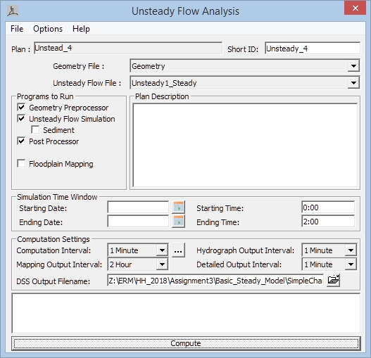
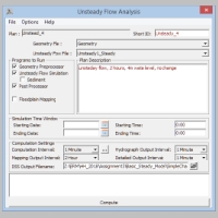
3.	perform the Unsteady Flow Analysis unsteady flow anlaysis form:	activate Geometry Preprocessor, Unsteady Flow Simulation and Post Processor set Starting Time to 00:00 set Ending Time to 02:00 set Computation Interval (time step) to 1 Minute set Hydrograph Output Interval to 1 Minute keep Mapping Output Interval on a high value (e.g. 2 hours, we are not generating maps) set Detailed Output Interval to 1 Minute save the Plan in a new file with suitable name finally run the simulation by the Compute button
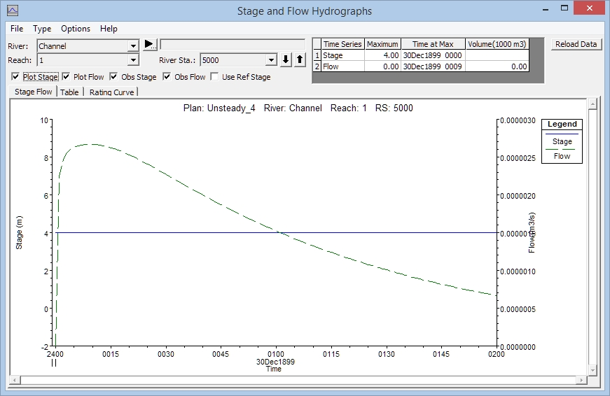
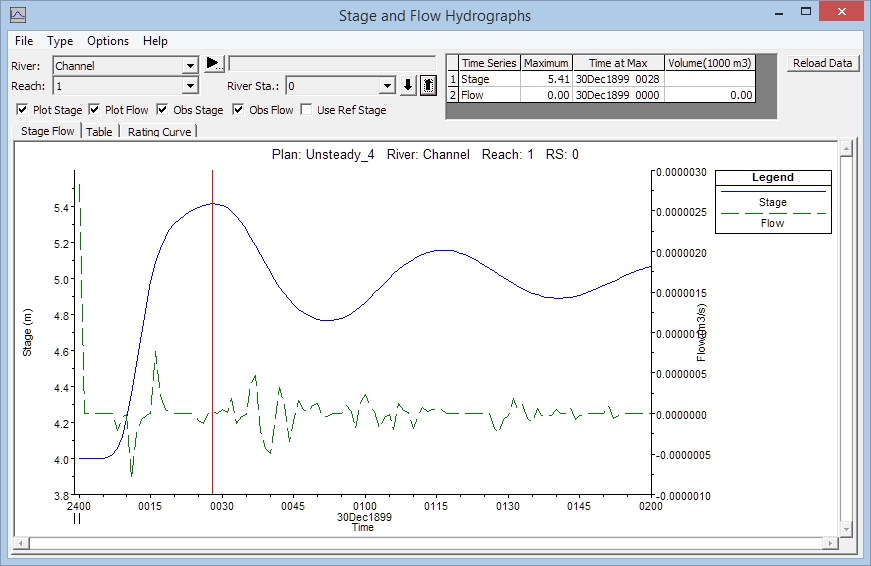
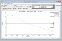
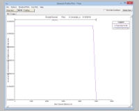
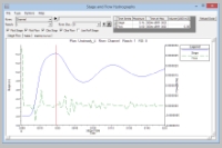
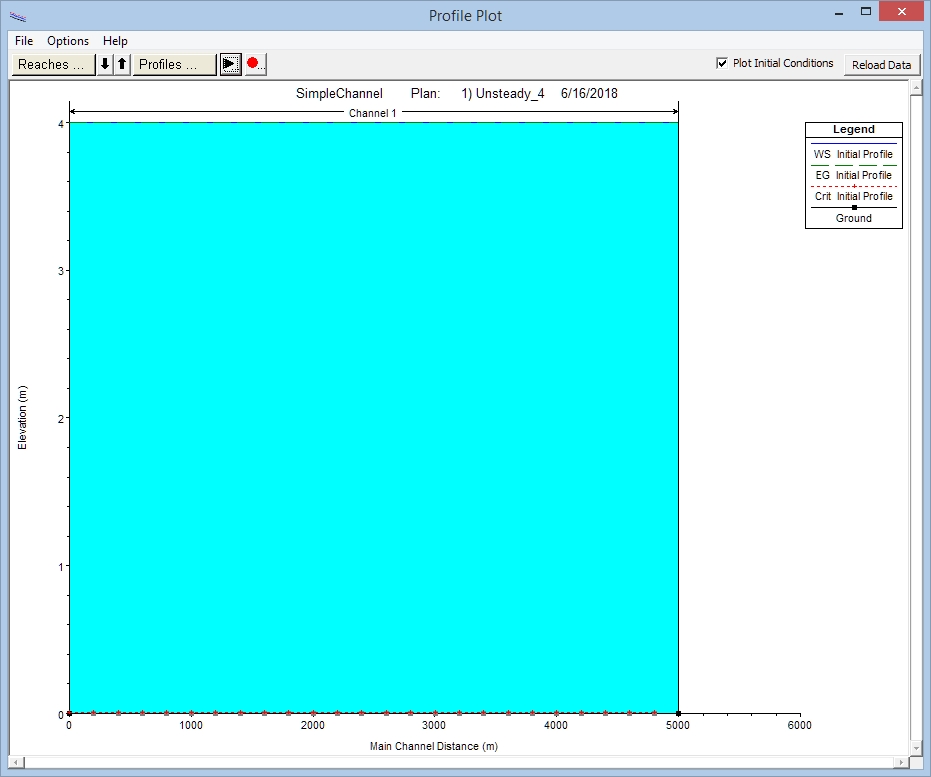
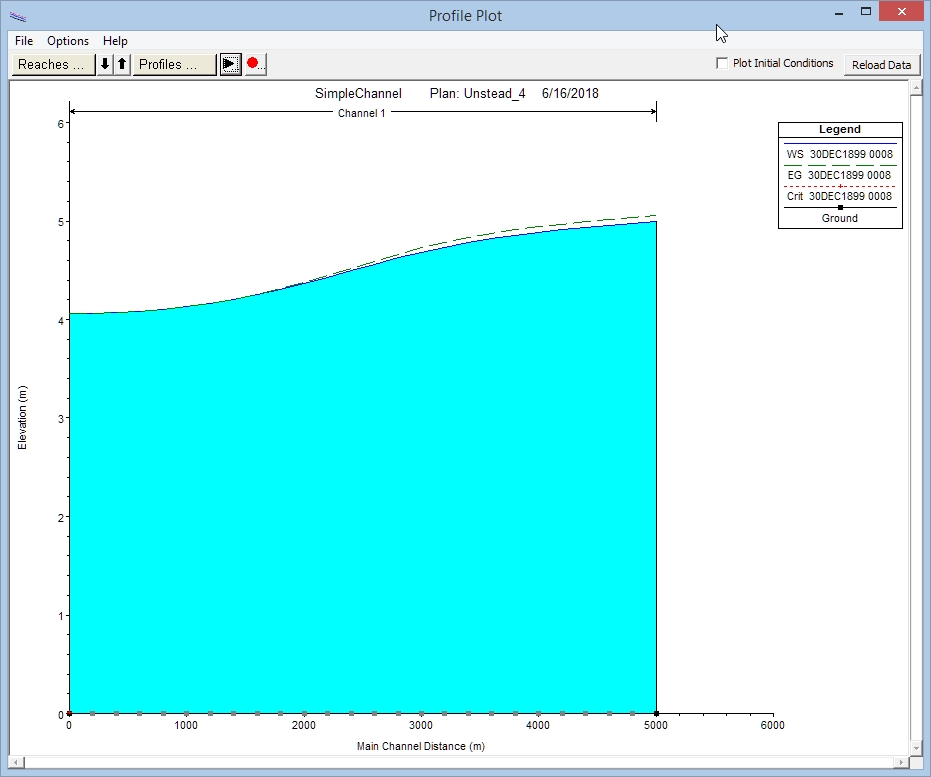
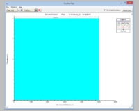
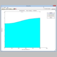
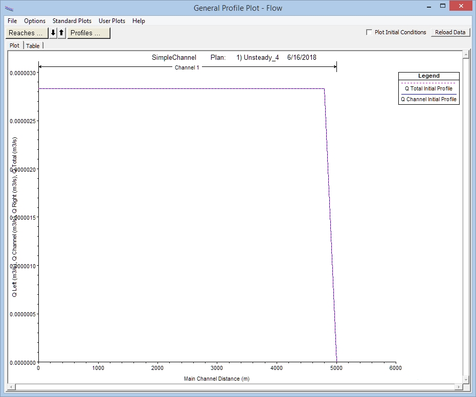
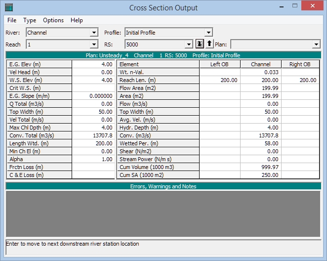
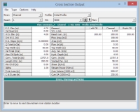
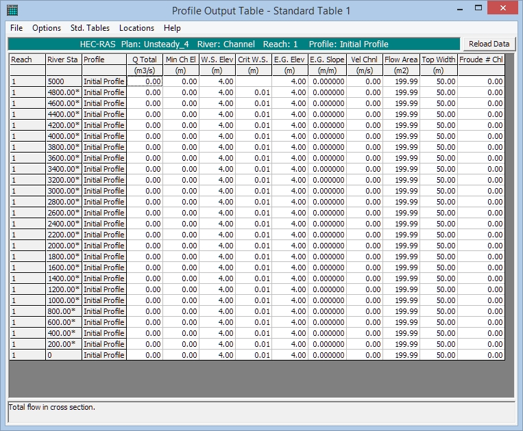
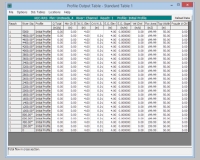
4.	analyse the results hydrograph diagram: profile plot: general profile: cross section table profile table:	use Stage and Flow Hydrographs to analyse the h(t) and Q(t) time series upstream and downstream use Water Surfave Profile to analyse the water surface in a longitudal profile h(x) use General Profile to analyse the result values R in a longitudal profile R(x) use Detailed Output Tables to get access to all relevant numbers for cross sections use Detailed Output Tables to get access to all simulation numbers in time and space
5.	initiate a wave stage hydrograph: profile plot: hydrograph diagram:	change the Stage Hydrograph upstream: increase the water surface elevation after 2 min from 4 m to 5 m analyse the results (step 4.) and specify the travel time of the wave from the result numbers compare your result analytic insight from hydraulics the speed of a gravity wave in shallow water is sqrt(gh) the time to run 5000 m is 5000 / sqrt(gh) for 4 m this is 5000 / sqrt(9.81*4) = 798 sec = 13,3 min

Step 3: Variation of the basic unsteady model

Please adapt your model with a variation of parameters.

change the upstream water surface elevation from 4m/5m to 8m/9m (1m -> wave height)
this requires the change of the Stage Hydrograph and the Inital Stage value of the Flow Hydrograph
and analyse the impact of the new water level ((8m)m instead of 4m )
to the travel time in the channel
change the cross section width 50 m to other values (e.g. 20 m or 100 m)
and analyse the impact to the results (e.g. hydrograph diagram)
change the calculation time step (1 sec, 10 sec, 5 min, 30 min)
and analyse the impact to the results (e.g. hydrograph diagram) using physical/numerical insight
change the cross section distance to 50 m and 1000 m (XS interpolation)
and analyse the impact to the results (e.g. hydrograph diagram) using physical/numerical insight

Optional/Volountary additional variations of parameter:

change the discharge at the boundary to introduce a basic velocity
introduce a slope for the channel
fix the water level and introduce a discharge time series
change the bed resistance values

Step 4: Result Discussion

Please compare and discuss the results of the basic unsteady model as well as the four variations with your expectations and the theory of open channel flow. The comparison and discussion (interpretation) should consider:

travel time of the wave to arrive at the other end of the channel
water level time series at station 0, station 2500 and station 5000
velocity and discharge time series at stations 0, 2500 and 5000
max. water level at station 0 vs. station 5000
numerical properties (e.g. time step, space step) of the model