
Pages: Assignment - Part 1 - Part 2
This is a step by step tutorial for the 1D hydraulic model HEC-RAS (Version 5.0.1) using the geometry and the flow data from the flood event at Nice (France) at Nov. 6th 1994.
The software download, graphical user interface and general workflow of HEC-RAS has already been introduced in the step by step tutorial for a prismatic channel of 5km length. If you have questions regarding these topics, please have a look there. You find the documentation on the course website.
IMPORTANT: Please switch your language and time/date settings of your computer to English (USA) before starting any HEC-RAS model. Also set default units within HEC-RAS to SI (international system of units) before loading any model.
Please download the Var.zip file from the course website. Extract the files.
Open HEC-RAS and load the project named Var. This steady state model includes the project file Var.prj, the plan file Var.p02, the geometry file Var_Geoemtry.g01 of the lower 24km of the river Var and the steady flow file Var_steady.f02 representing the base flow, as can be seen in figure 1.
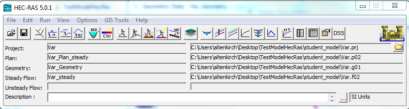
Figure 1: Steady Var model
Please have a look at the geometry data. You may use the Plot XYZ option (right click on river) to view the entire river section or view the individual cross sections. A uniform Manning roughness coefficient of 0.033 has been assumed for all sections of the river and embankments.

Please have a look at the steady flow data. This steady model uses a constant upstream discharge of 300m3/s with a normal depth for an energy gradient of 0.03 and a rating curve (Q-H relationship) for a free outflow at the downstream reach 0. You will find the same rating curve in the provided excel file in the Var.zip folder.

Please have a look at the steady flow
simulation data. Note, that the mixed flow regime option is selected as the
river does have large changes in the geometry and therefore potentially also in
the flow regime.
Please run the steady model again now.

Please use the post processing viewing options to get a feeling for the steady base flow conditions. For example the longitudinal profile. Here, under Options -> Variables you can view a number of helpful parameter, e.g. the elevations of the left and right river banks, water surface, energy grade line etc.
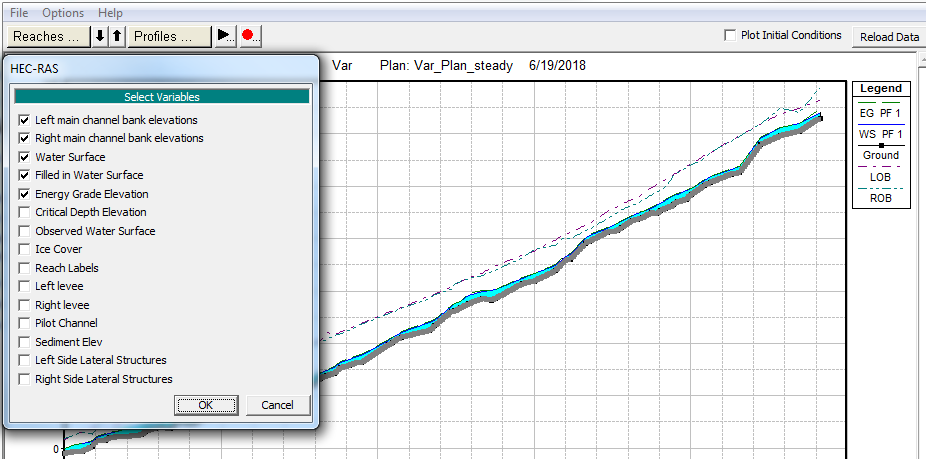
Figure 2: Variables for longitudinal profile plotting
You should also have a look at the summary table of all profiles Here you can notice, that the flow regime changes between sub- and supercritical depending on the channel slope and geometry, with some river sections even being very close to critical flow conditions. The dominant flow regime is supercritical flow, as could be expected from a steep mountainous river such as the river Var.
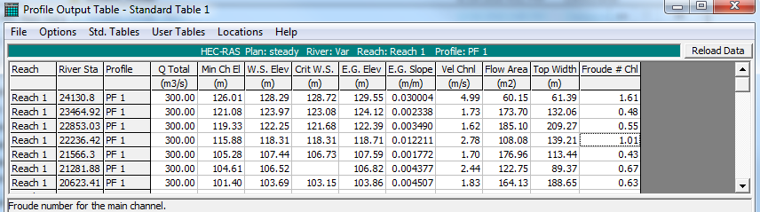
Figure 3: Profile output table
Before creating the unsteady model of the actual flood event, the initial conditions can be generated with the help of a hotstart. Please create a new unsteady flow data file called hotstart.
For the upstream boundary (RS: 24130.8), please use a flow hydrograph with constant hourly values of 300m3/s for the time period between the (fixed starting time) 4th November 1994 1:00AM and the 5th November 1994 1:00AM. To create a hotstart, it is recommended to use at least 24h. You can copy the discharge data from the Excel sheet (spreadsheet: BC hotstart) or fill the table manually using the interpolating missing values option. Make sure that the correct starting date and time is set (figure 4).
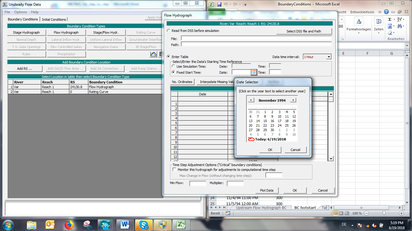
Figure 4: Setting a fixed Start Time for an unsteady simulation
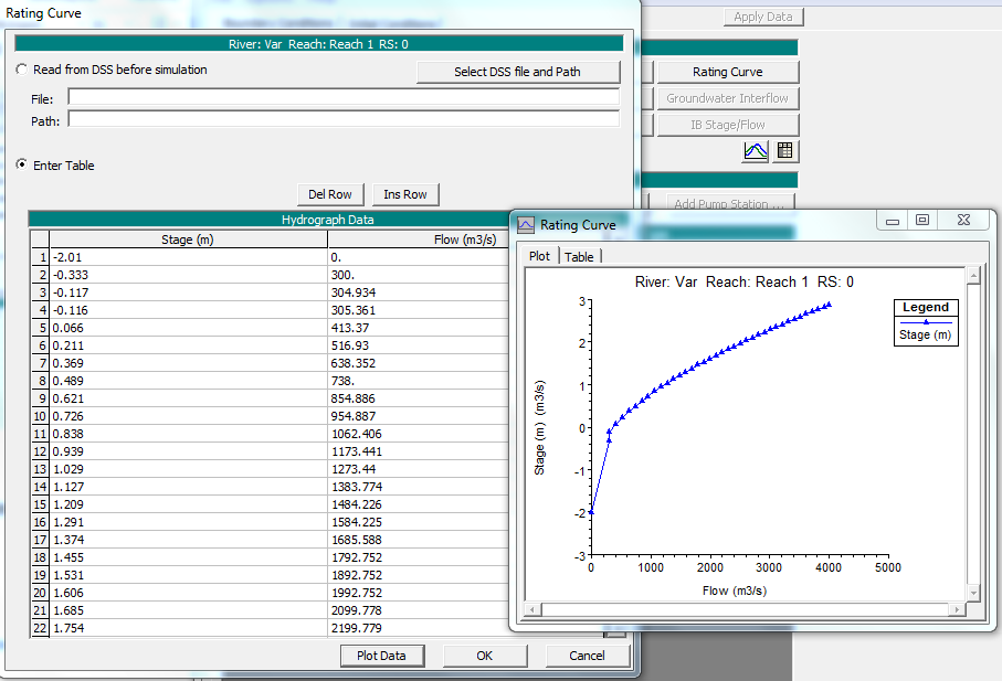
Figure 5: Rating Curve table and plotted data
After the upstream boundary condition, the downstream boundary condition has to be defined. For this, we use the same rating curve as for the steady simulation. You may copy the Q-H values from the provided excel sheet (spreadsheet: Downstream RatingCurve Bc) and plot the data (see figure 5)
After the boundary conditions, the initial conditions have to be defined. We would like to use the results from the steady state simulation to define the initial conditions.
File-> Set initial conditions (flow and stage) from previous output profile ...
Choose the file Var_Plan_steady from the dropdown menu and overwrite the current default condition for the initial time step. If not yet done, save your flow data file as hotstart.

Open the Unsteady flow analysis window and create a new plan called hotstart with the short identifier ID hotstart
For the simulation, use the original geometry file Var_Geometry and the unsteady flow file hotstart. Please activate the geometry preprocessor, unsteady flow simulation and post processor and enter the 4th November 1994 1:00AM as starting Date and the 5th November 1994 1:00AM as ending date. The computation interval should be 10 seconds and the output intervals each 1 hour. As during the steady flow, the flow regime will have to be computed as mixed flow regimes.
Options -> Computation Options and Tolerances -> 1D Mixed Flow Options -> Activate -> OK
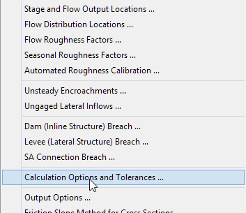
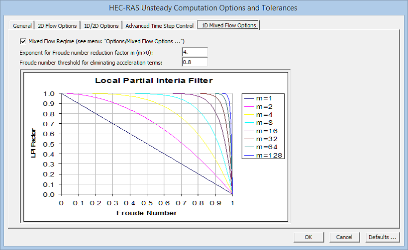
Figure 6: Mixed Flow Regime option (HEC-RAS Version 5.0.4)
Please Note! If you have an older version of HEC-RAS (e.g. 5.0.1), the flow mixed option is directly be activated in the computing window, as can be seen in the figure 7 below. View the figure below!
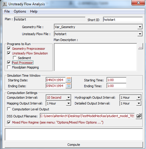
Figure 7: Simulation settings for the hotstart simulation (based on HEC-RAS 5.0.1)
Now create a new unsteady file called unsteady. Please use a flow hydrograph for upstream using the data given in the excel sheet (spreadsheet: Upstream Flow hydrograph) using the same starting time as before and the same rating curve for the downstream boundary condition (spreadsheet: Downstream RatingCurve BC).
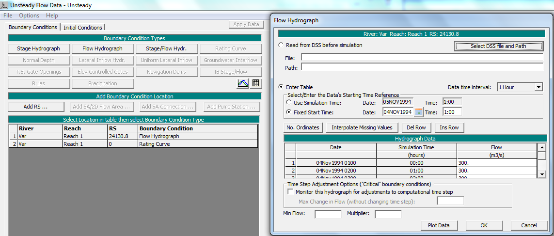
Figure 8: Unsteady Flow data and flow hydrograph using fixed starting time
For the initial condition we will now use the results from the hotstart file.
File -> Set initial conditions (flow and stage) from previous output profile . . . -> hotstart
Choose the file hotstart from the dropdown menu and the maximum water surface (Max WS) from that simulation. You may overwrite the current default condition for the initial time step.
Please open the Unsteady flow analysis window and create a new plan called Unsteady and the short identifier ID unsteady,
The simulation should now start on the 5th November 1994 1:00AM and continue until the 8th November 1994 1:00AM. The computational interval should be 10 seconds, while the hydrograph and detailed output interval should be 30 minutes. The mapping hydrograph can remain as 1 hour. Make sure to check the mixed flow regime option. View the figure below!
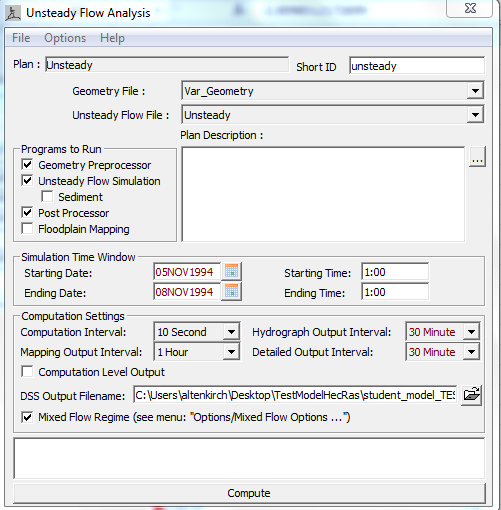
Figure 9: Simulation file for the unsteady flood simulation
As described before, in newer HEC-RAS versions, the mixed flow regime option is activated as follows:
Options -> Calculation Options and Tolerances -> 1D Mixed Flow Options -> Activate -> OK
Using the post processing tools, that you already know, please answer the following questions:
You may have noticed already, that there is another geometry file called Var_weir. This geometry file contains 6 weirs. Please create a new unsteady plan file called Weir_unsteady, in which you use the same settings as before, only change the geometry file from Var_geometry to Var_weir. (see Figure)
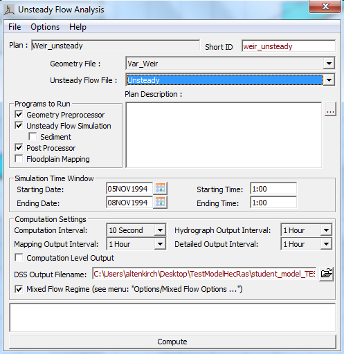
Figure 10: Simulation file for flood simulation with weirs
After the run, please have a look at your results (e.g. Figure 11) and answer the following questions:
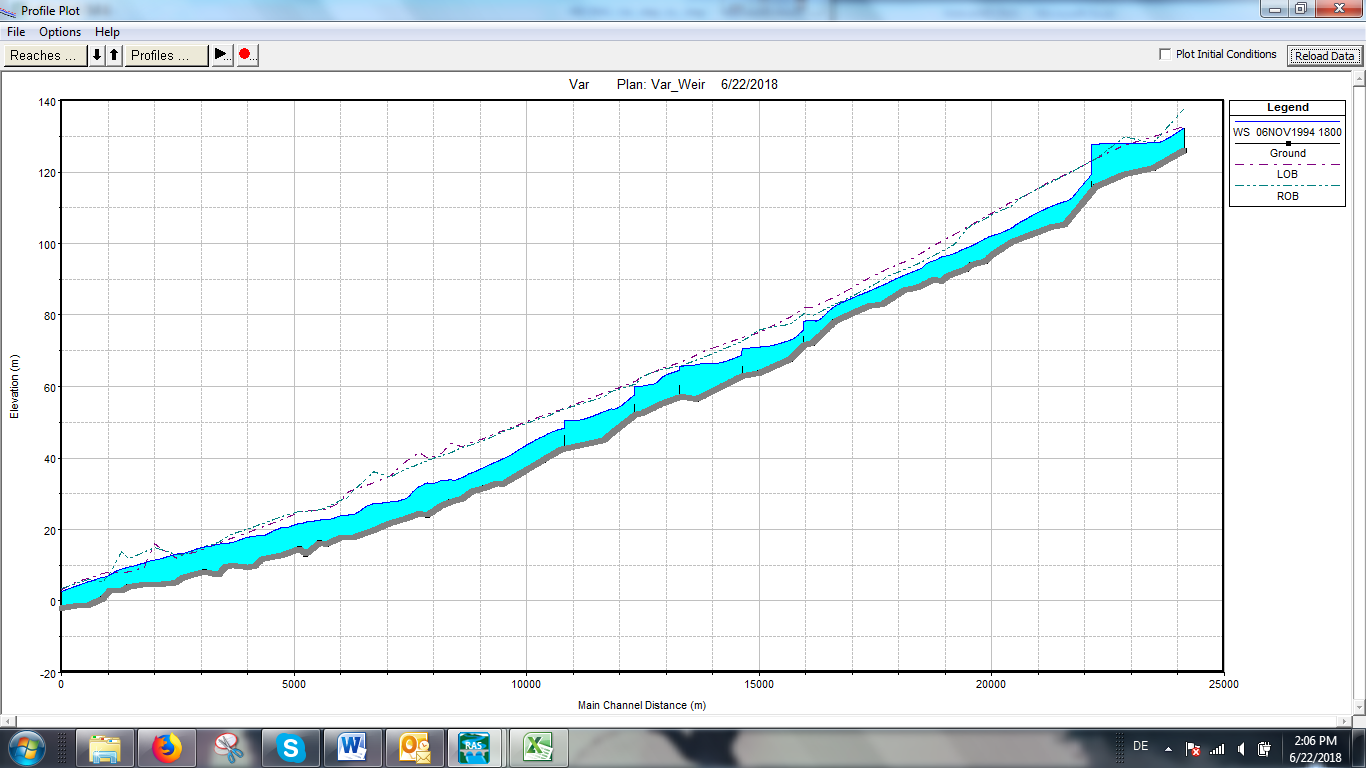
Figure 11: Longitudinal profile of the river Var including the weirs
at the
time of the peak discharge at 6.Nov 1994 18:00
Please note:
Minor instabilities at the beginning of the simulation with the
weir geometry could occur, since we are using the initial conditions from a
geometry file that contains no weirs. As they only affect the very beginning of
your simulation, they are not severe, as we are more interested in the water
levels during the flood event and not at the beginning of the simulation.
However, if you would like to avoid these instabilities, we recommend you to follow the same work flow as before: